How Borůvka MST Works in HDBSCAN

From the 1926 algorithm to dual-tree pruning — and why the MST structure drives cluster counts

← Back to Rhobots

HDBSCAN requires a minimum spanning tree (MST) of the mutual reachability distance graph. At small corpus sizes that MST is trivial to compute; at 10,000+ documents the naive approach requires an \(O(n^2)\) distance matrix — roughly 100 GB of RAM at \(n = 100{,}000\).

Rhobots solves this with the Borůvka algorithm (Otakar Borůvka, 1926), augmented with a Ball-tree or KD-tree spatial index so each round of the algorithm runs in \(O(n \log n)\) instead of \(O(n^2)\).

This page explains every layer: what an MST is, how Borůvka builds one in rounds, how a dual-tree spatial index prunes most of the work, and — critically — why different MST algorithms can produce structurally different trees on diffuse data, which is the root cause of cluster-count variation between implementations.

---

1 The Minimum Spanning Tree

A spanning tree of \(n\) points is a set of \(n - 1\) edges that connects every point to every other (directly or indirectly) with no cycles. There are exponentially many spanning trees of a complete graph; the minimum spanning tree is the one with the smallest total edge weight.

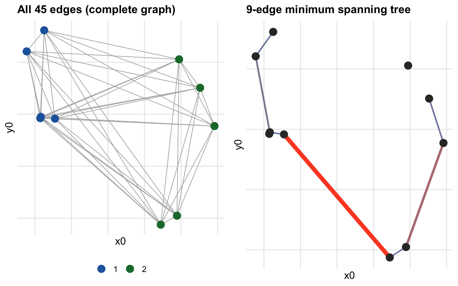
In the HDBSCAN context each edge weight is the mutual reachability distance (MRD) between the two endpoints (explained in Section 3). The MST of the MRD graph captures the essential density skeleton of the data: low-weight edges sit inside dense clusters; high-weight edges cross the sparse gaps between clusters.

set.seed(42)
n_toy <- 10
X10   <- rbind(
  cbind(rnorm(5, -2, 0.4), rnorm(5, 0, 0.4)),
  cbind(rnorm(5,  2, 0.4), rnorm(5, 0, 0.4))
)
grp10 <- rep(c("1","2"), each = 5)
D10   <- as.matrix(dist(X10))

# Prim's MST on D10
prim_mst <- function(W) {
  n <- nrow(W); in_mst <- logical(n); in_mst[1] <- TRUE
  edges <- matrix(0L, n-1, 2); ws <- numeric(n-1)
  key <- rep(Inf, n); parent <- integer(n)
  key[1] <- 0
  for (step in seq_len(n-1)) {
    u <- which.min(ifelse(in_mst, Inf, key))
    in_mst[u] <- TRUE; edges[step,] <- c(parent[u], u); ws[step] <- key[u]
    for (v in which(!in_mst)) if (W[u,v] < key[v]) { key[v] <- W[u,v]; parent[v] <- u }
  }
  list(edges = edges[-1,,drop=FALSE], w = ws[-1])
}
mst10 <- prim_mst(D10)

all_e <- do.call(rbind, lapply(1:(n_toy-1), function(i) {
  do.call(rbind, lapply((i+1):n_toy, function(j) {
    data.frame(x0=X10[i,1],y0=X10[i,2],x1=X10[j,1],y1=X10[j,2],w=D10[i,j])
  }))
}))
mst_e <- data.frame(
  x0 = X10[mst10$edges[,1],1], y0 = X10[mst10$edges[,1],2],
  x1 = X10[mst10$edges[,2],1], y1 = X10[mst10$edges[,2],2], w = mst10$w
)
pts10 <- data.frame(x=X10[,1], y=X10[,2], g=grp10)

p_all <- ggplot() +
  geom_segment(data=all_e, aes(x=x0,y=y0,xend=x1,yend=y1), colour="grey70", linewidth=0.4) +
  geom_point(data=pts10, aes(x,y,colour=g), size=4) +
  scale_colour_manual(values=PAL) +
  labs(title="All 45 edges (complete graph)", colour=NULL)

p_mst <- ggplot() +
  geom_segment(data=mst_e, aes(x=x0,y=y0,xend=x1,yend=y1,linewidth=w,colour=w)) +
  geom_point(data=pts10, aes(x,y), colour="grey20", size=4) +
  scale_colour_gradient(low="#4292C6", high="#FC4E2A", guide="none") +
  scale_linewidth_continuous(range=c(0.6,2.5), guide="none") +
  labs(title="9-edge minimum spanning tree")

grid.arrange(p_all, p_mst, ncol=2)

Left: all possible edges on 10 points (complete graph, 45 edges). Right: the MST — 9 edges that connect every point with minimum total weight. Heavy edges cross the gap between the two groups.

The heaviest MST edge separates the two groups. Cutting that edge at the right \(\lambda\) level is precisely how HDBSCAN identifies cluster boundaries.

---

2 Why Not Prim’s or Kruskal’s?

All three classical MST algorithms produce the same MST on a complete graph with distinct edge weights. Their differences are computational, not mathematical.

Algorithm	Strategy	Memory	Time
Prim’s	Greedy: always add cheapest edge to growing tree	\(O(n^2)\) distances	\(O(n^2)\)
Kruskal’s	Sort all edges; add if they connect different components	\(O(n^2)\) edges	\(O(n^2 \log n)\)
Borůvka’s	Parallel: every component finds its cheapest outgoing edge simultaneously	\(O(n \cdot k)\)	\(O(n \log n)\) rounds

The critical column is memory. Prim’s needs to compare every candidate edge against every already-selected point, which means holding all \(n^2/2\) pairwise distances in RAM. At \(n = 30{,}000\) and 8 bytes per double, that is \(\approx 3.6\) GB — already beyond a typical laptop. At \(n = 100{,}000\) it is \(\approx 40\) GB.

Borůvka avoids this because each round only ever asks: “What is the cheapest edge leaving my current component?” That question can be answered from a \(k\)-nearest-neighbour graph, which costs only \(O(n \cdot k)\) to store.

---

3 Mutual Reachability Distance (recap)

Before Borůvka can run, HDBSCAN defines a modified distance that rewards density. The mutual reachability distance between points \(x_i\) and \(x_j\) is:

\[d_{\text{mrd}}(i, j) = \max\bigl\{\text{core}(i),\; \text{core}(j),\; d(i, j)\bigr\}\]

where \(\text{core}(i)\) is the distance from \(i\) to its min_pts-th nearest neighbour.

Three cases:

Situation	MRD value
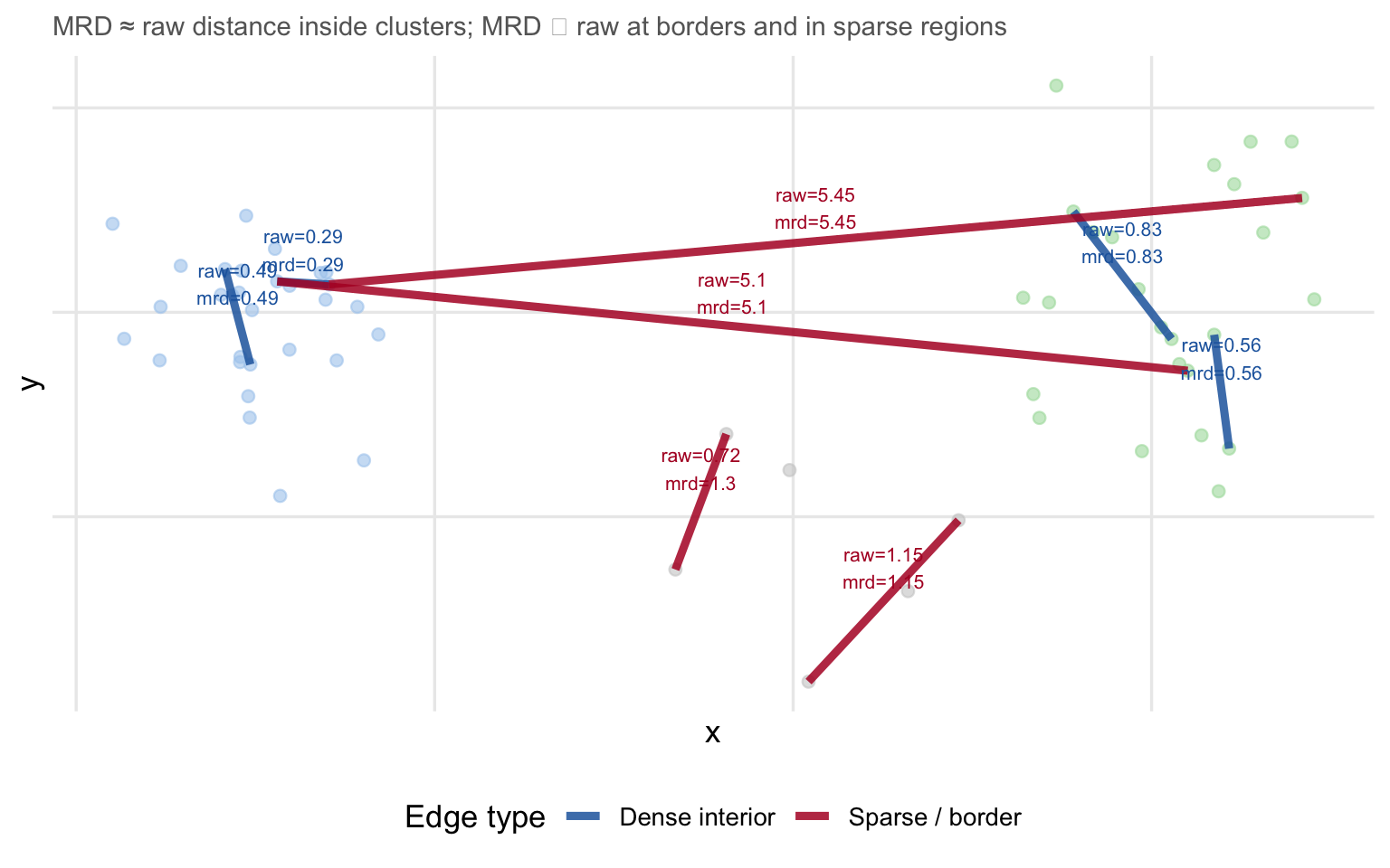
Both points in a dense cluster	\(\approx d(i,j)\) — core distances small, raw distance dominates
One point on cluster border	\(\approx \text{core}(\text{border point})\) — core distance of the sparse point dominates
Both points in sparse region	\(\approx \max(\text{core}(i), \text{core}(j)) \gg d(i,j)\) — MRD far exceeds raw distance

This inflation of sparse-region edges is what causes HDBSCAN to draw sharp cluster boundaries even in the absence of a clear raw-distance gap.

set.seed(42)
g1  <- cbind(rnorm(30, -3,  0.3), rnorm(30,  0, 0.3))
g2  <- cbind(rnorm(25,  2,  0.6), rnorm(25,  0, 0.6))
ns  <- cbind(runif(6, -1, 1),     runif(6, -2, 2))
X_m <- rbind(g1, g2, ns)
n_m <- nrow(X_m)

D_m    <- as.matrix(dist(X_m))
knn_m  <- t(apply(D_m, 1, function(r) order(r)[2:6]))
core_m <- D_m[cbind(seq_len(n_m), knn_m[,4])]  # 4th NN = core(min_pts=4)

mrd_fn <- function(i, j) max(core_m[i], core_m[j], D_m[i,j])

# Sample some edges to illustrate
in_edge  <- list(c(1,5), c(2,8), c(32,35), c(33,40))
out_edge <- list(c(58,59), c(57,60), c(5,37), c(1,34))

draw_edge <- function(e, type) {
  data.frame(x0=X_m[e[1],1], y0=X_m[e[1],2],
             x1=X_m[e[2],1], y1=X_m[e[2],2],
             raw=round(D_m[e[1],e[2]],2),
             mrd=round(mrd_fn(e[1],e[2]),2),
             type=type)
}
edge_df <- rbind(
  do.call(rbind, lapply(in_edge,  function(e) draw_edge(e, "Dense interior"))),
  do.call(rbind, lapply(out_edge, function(e) draw_edge(e, "Sparse / border")))
)
pts_m <- data.frame(x=X_m[,1], y=X_m[,2],
                     g=c(rep("1",30),rep("2",25),rep("noise",6)))

ggplot() +
  geom_point(data=pts_m, aes(x,y,colour=g), size=2, alpha=0.6) +
  geom_segment(data=edge_df,
               aes(x=x0,y=y0,xend=x1,yend=y1,colour=type),
               linewidth=1.6, alpha=0.85) +
  scale_colour_manual(
    values=c("1"="#AACCEE","2"="#AADDAA","noise"="#CCCCCC",
             "Dense interior"="#2166AC","Sparse / border"="#B2182B"),
    breaks=c("Dense interior","Sparse / border"),
    name="Edge type") +
  geom_text(data=edge_df,
            aes(x=(x0+x1)/2, y=(y0+y1)/2,
                label=paste0("raw=",raw,"\nmrd=",mrd), colour=type),
            size=2.8, vjust=-0.3, show.legend=FALSE) +
  labs(subtitle="MRD ≈ raw distance inside clusters; MRD ≫ raw at borders and in sparse regions")

Effect of MRD on edge weights. Red edges connect points in sparse regions — their MRD far exceeds the raw Euclidean distance. Blue edges connect dense-cluster interiors where MRD ≈ raw distance.

---

4 Borůvka’s Algorithm Step by Step

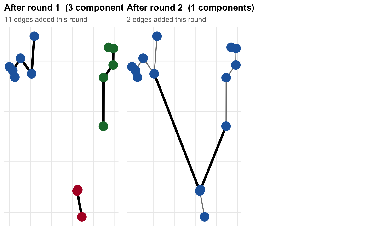
Borůvka works in rounds. Each round does two things:

1. Every current component independently finds the cheapest edge that leads out of it (a best outgoing edge).
2. All those edges are added to the MST simultaneously, merging components.

After each round the number of components is at least halved, so at most \(\lceil \log_2 n \rceil\) rounds are needed.

set.seed(5)
n_b <- 14
X_b <- rbind(
  cbind(rnorm(6, -2.5, 0.4), rnorm(6,  1.0, 0.4)),
  cbind(rnorm(5,  2.0, 0.5), rnorm(5,  0.8, 0.5)),
  cbind(rnorm(3,  0.0, 0.3), rnorm(3, -2.0, 0.3))
)
D_b <- as.matrix(dist(X_b))

# Prim's MST on this graph
mst_b <- prim_mst(D_b)

# Borůvka simulation (on full distance matrix for illustration)
boruvka_sim <- function(W) {
  n   <- nrow(W)
  par <- seq_len(n)   # par[i] = component root of i

  find <- function(x) { while (par[x] != x) { par[x] <<- par[par[x]]; x <- par[x] }; x }
  unite <- function(a, b) {
    ra <- find(a); rb <- find(b)
    if (ra == rb) return(FALSE)
    par[rb] <<- ra; TRUE
  }

  all_edges <- list()   # accumulate added edges by round
  all_comps <- list()   # component assignment by round

  repeat {
    comps <- sapply(seq_len(n), find)
    if (length(unique(comps)) == 1) break

    bw <- rep(Inf, n); bu <- rep(-1L, n); bv <- rep(-1L, n)

    for (i in seq_len(n)) {
      ci <- find(i)
      for (j in seq_len(n)) {
        cj <- find(j)
        if (ci == cj) next
        if (W[i,j] < bw[ci]) { bw[ci] <- W[i,j]; bu[ci] <- i; bv[ci] <- j }
      }
    }

    round_edges <- list()
    for (r in unique(comps)) {
      if (bu[r] < 0) next
      if (unite(bu[r], bv[r])) {
        round_edges <- c(round_edges, list(c(bu[r], bv[r], bw[r])))
      }
    }
    all_comps <- c(all_comps, list(sapply(seq_len(n), find)))
    all_edges <- c(all_edges, list(round_edges))
  }
  list(comps = all_comps, edges = all_edges)
}

sim <- boruvka_sim(D_b)

# Helper: accumulated MST edges up to round r
cum_edges <- function(r) {
  do.call(rbind, unlist(sim$edges[seq_len(r)], recursive=FALSE))
}

# Remap component IDs to sequential integers for colour mapping
remap_comps <- function(comps) {
  m <- match(comps, sort(unique(comps)))
  m
}

n_rounds <- length(sim$comps)
plots <- lapply(seq_len(n_rounds), function(r) {
  comp_r   <- remap_comps(sim$comps[[r]])
  n_comps  <- max(comp_r)
  pts_df   <- data.frame(x=X_b[,1], y=X_b[,2], comp=factor(comp_r))

  # Accumulated MST edges (added in rounds 1..r)
  mst_so_far <- if (r == 1) NULL else {
    m <- cum_edges(r - 1)
    if (is.null(m)) NULL else
      data.frame(x0=X_b[m[,1],1], y0=X_b[m[,1],2],
                 x1=X_b[m[,2],1], y1=X_b[m[,2],2])
  }

  # Edges added THIS round
  this_round <- do.call(rbind, sim$edges[[r]])
  new_e <- if (!is.null(this_round))
    data.frame(x0=X_b[this_round[,1],1], y0=X_b[this_round[,1],2],
               x1=X_b[this_round[,2],1], y1=X_b[this_round[,2],2])
  else NULL

  comp_pal <- setNames(
    c("#2166AC","#1B7837","#B2182B","#762A83","#E08214","#01665E",
      "#8C510A","#4D4D4D","#F6E8C3","#D1E5F0","#FDDBC7","#D9F0A3","#E7D4E8"),
    as.character(seq_len(13))
  )

  p <- ggplot() +
    { if (!is.null(mst_so_far))
        geom_segment(data=mst_so_far,
                     aes(x=x0,y=y0,xend=x1,yend=y1),
                     colour="grey50", linewidth=0.8) } +
    { if (!is.null(new_e))
        geom_segment(data=new_e,
                     aes(x=x0,y=y0,xend=x1,yend=y1),
                     colour="black", linewidth=1.8) } +
    geom_point(data=pts_df, aes(x,y,colour=comp,fill=comp),
               size=5, shape=21, stroke=1.5) +
    scale_colour_manual(values=comp_pal, guide="none") +
    scale_fill_manual(values=comp_pal, guide="none") +
    labs(title=sprintf("After round %d  (%d components)", r, n_comps),
         subtitle=sprintf("%d edges added this round",
                          length(sim$edges[[r]])),
         x=NULL, y=NULL)
  p
})

do.call(grid.arrange, c(plots, ncol=3))

Borůvka in action on 14 points. Each panel shows the state after one round. Colours identify components; solid lines are newly added MST edges; dashed lines show each component’s cheapest outgoing edge that will be added. By round 3 all points are connected.

Reading the diagram. Each colour is one component. Black edges are newly added in that round; grey edges were added earlier. Notice that in Round 1 every individual point acts alone — 14 independent searches. After Round 1 components have formed and the next search covers entire groups. By Round 3 a single component spans all 14 points: the MST is complete.

---

5 Union-Find: Tracking Components in O(α(n))

Borůvka needs to answer two questions millions of times per run:

• Which component does point \(i\) belong to? (find)
• Merge the components of \(i\) and \(j\). (unite)

A naïve implementation rescans all points at each query (\(O(n)\)). The Union-Find data structure answers both in effectively \(O(1)\) amortised time using two tricks:

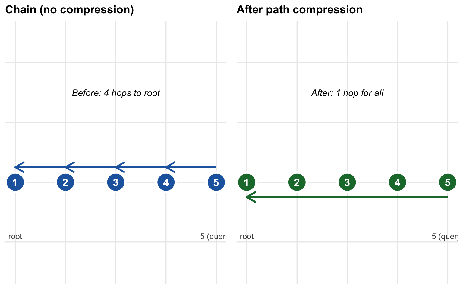
Path compression (in find). While walking up the parent-pointer chain to the root, reattach every visited node directly to the root. Future queries on those nodes skip the chain entirely.

Union by size (in unite). Always attach the smaller tree under the root of the larger tree. This bounds the tree height at \(O(\log n)\), preventing degenerate chains.

Together these give amortised \(O(\alpha(n))\) per operation, where \(\alpha\) is the inverse Ackermann function — for all practical \(n\) it is less than 5.

# Diagram: chain of 5 nodes before/after path compression
node_pos <- data.frame(
  id  = 1:5,
  x   = c(0, 1, 2, 3, 4),
  y   = c(0, 0, 0, 0, 0),
  lab = c("root", "2", "3", "4", "5 (query)")
)
arrows_before <- data.frame(
  x0  = c(1,2,3,4), y0 = 0.05,
  x1  = c(0,1,2,3), y1 = 0.05
)
arrows_after <- data.frame(
  x0 = c(1,2,3,4), y0 = -0.05,
  x1 = c(0,0,0,0), y1 = -0.05
)

p_before <- ggplot() +
  geom_segment(data=arrows_before,
               aes(x=x0,y=y0,xend=x1,yend=y1),
               arrow=arrow(length=unit(0.18,"inches")),
               linewidth=1, colour="#2166AC") +
  geom_point(data=node_pos, aes(x,y), size=10, colour="white",
             fill="#2166AC", shape=21, stroke=2) +
  geom_text(data=node_pos, aes(x,y,label=id), colour="white", fontface="bold") +
  geom_text(data=node_pos[c(1,5),], aes(x,y-0.18,label=lab),
            colour="grey30", size=3.5) +
  annotate("text",x=2,y=0.3,label="Before: 4 hops to root",size=4,fontface="italic") +
  coord_cartesian(ylim=c(-0.3,0.5)) +
  labs(title="Chain (no compression)", x=NULL, y=NULL)

p_after <- ggplot() +
  geom_segment(data=arrows_after,
               aes(x=x0,y=y0,xend=x1,yend=y1),
               arrow=arrow(length=unit(0.18,"inches")),
               linewidth=1, colour="#1B7837") +
  geom_point(data=node_pos, aes(x,y), size=10, colour="white",
             fill="#1B7837", shape=21, stroke=2) +
  geom_text(data=node_pos, aes(x,y,label=id), colour="white", fontface="bold") +
  geom_text(data=node_pos[c(1,5),], aes(x,y-0.18,label=lab),
            colour="grey30", size=3.5) +
  annotate("text",x=2,y=0.3,label="After: 1 hop for all",size=4,fontface="italic") +
  coord_cartesian(ylim=c(-0.3,0.5)) +
  labs(title="After path compression", x=NULL, y=NULL)

grid.arrange(p_before, p_after, ncol=2)

Path compression in action. Before (left): a chain of 5 nodes requires 5 hops to find the root. After one find() call with path compression (right): all nodes now point directly to the root. Future queries cost O(1).

---

6 The kNN Approximation

A complete MRD graph has \(n(n-1)/2\) edges — the same \(O(n^2)\) problem that kills Prim’s. Borůvka avoids this by restricting each point to only looking at its \(k\) nearest Euclidean neighbours when searching for its component’s cheapest outgoing edge.

This is an approximation. The key question is whether the true MST ever requires an edge that goes to a point beyond the \(k\)-th nearest Euclidean neighbour.

For standard Euclidean data with distinct distances: no. The optimal outgoing edge from any component always connects to one of the \(k\) nearest Euclidean neighbours of some component member, as long as \(k \geq \text{min\_pts}\).

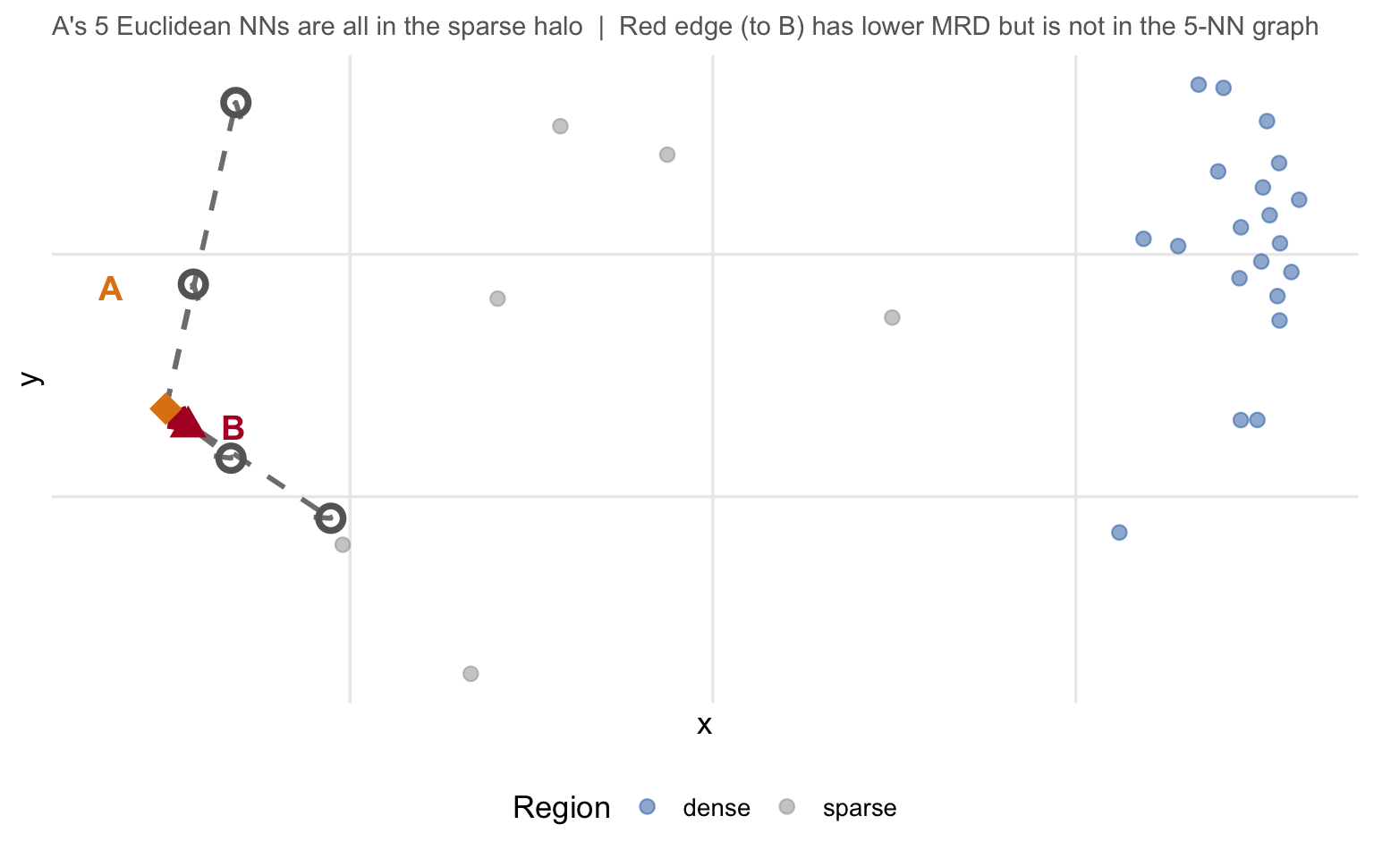
For MRD on diffuse embeddings: occasionally yes. A point \(j\) that is the 20th Euclidean neighbour of \(i\) might have a smaller MRD to \(i\) than any of the 15 nearest Euclidean neighbours, if \(j\) sits in a dense sub-region (small core distance) while the 15 nearest neighbours all sit in sparse areas (large core distances, inflating MRD).

set.seed(99)
dense_cl  <- cbind(rnorm(20,  3, 0.25), rnorm(20, 0, 0.25))
sparse_cl <- cbind(rnorm(12, -1, 1.2),  rnorm(12, 0, 0.8))
X_km <- rbind(dense_cl, sparse_cl)
n_km <- nrow(X_km)
D_km <- as.matrix(dist(X_km))

# min_pts = 6 → core = 6th NN
core_km <- apply(D_km, 1, function(r) sort(r)[7])
mrd_km  <- function(i,j) max(core_km[i], core_km[j], D_km[i,j])

# "A" = the outer isolated point (last of sparse_cl)
# Pick A as the point farthest from the dense cluster among sparse
A_idx <- which.max(D_km[, 1])   # farthest from dense cluster centre (point 1)
nn_A  <- order(D_km[A_idx,])[2:9]   # 8 nearest Euclidean neighbours

# True min-MRD neighbour
mrd_vals <- sapply(nn_A, function(j) mrd_km(A_idx, j))
best_j   <- nn_A[which.min(mrd_vals)]

pts_km <- data.frame(x=X_km[,1], y=X_km[,2],
                      g=c(rep("dense",20), rep("sparse",12)))
pts_km$role <- "other"
pts_km$role[A_idx]  <- "A"
pts_km$role[nn_A[1:5]] <- "5-NN"
pts_km$role[best_j] <- "B (best MRD)"

seg_5nn <- data.frame(
  x0=X_km[A_idx,1], y0=X_km[A_idx,2],
  x1=X_km[nn_A[1:5],1], y1=X_km[nn_A[1:5],2]
)
seg_best <- data.frame(
  x0=X_km[A_idx,1], y0=X_km[A_idx,2],
  x1=X_km[best_j,1], y1=X_km[best_j,2]
)

ggplot() +
  geom_point(data=subset(pts_km, role=="other"),
             aes(x,y,colour=g), size=2.5, alpha=0.5) +
  geom_segment(data=seg_5nn,
               aes(x=x0,y=y0,xend=x1,yend=y1),
               colour="grey50", linewidth=1,
               arrow=arrow(length=unit(0.1,"in")), linetype="dashed") +
  geom_segment(data=seg_best,
               aes(x=x0,y=y0,xend=x1,yend=y1),
               colour="#B2182B", linewidth=2,
               arrow=arrow(length=unit(0.12,"in"))) +
  geom_point(data=subset(pts_km, role=="5-NN"),
             aes(x,y), colour="grey40", size=3.5, shape=1, stroke=2) +
  geom_point(data=subset(pts_km, role=="A"),
             aes(x,y), colour="#E08214", size=6, shape=18) +
  geom_point(data=subset(pts_km, role=="B (best MRD)"),
             aes(x,y), colour="#B2182B", size=5, shape=17) +
  scale_colour_manual(values=c(dense="#2166AC", sparse="#999999"),
                      name="Region") +
  annotate("text", x=X_km[A_idx,1]-0.3, y=X_km[A_idx,2]+0.25,
           label="A", colour="#E08214", fontface="bold", size=5) +
  annotate("text", x=X_km[best_j,1]+0.25, y=X_km[best_j,2],
           label="B", colour="#B2182B", fontface="bold", size=5) +
  labs(subtitle=paste0("A's 5 Euclidean NNs are all in the sparse halo  |  ",
                       "Red edge (to B) has lower MRD but is not in the 5-NN graph"))

Scenario where kNN misses the optimal MRD edge. Point A’s 5 nearest Euclidean neighbours (grey arrows) are all in the sparse halo. The true minimum-MRD edge (red) goes to point B — the 8th Euclidean neighbour — which sits inside a dense cluster and has a small core distance. With k=5 this edge is never considered.

Rhobots handles this with the dual-tree Borůvka approach: instead of restricting to a pre-built kNN list, it searches the entire dataset using a spatial tree and prunes only pairs whose MRD lower bound already exceeds the current best. No valid edge is missed.

---

7 Dual-Tree Borůvka with a Ball-tree

The naive Borůvka step — for every component, scan all other components — costs \(O(n^2)\) per round. Dual-tree Borůvka brings this down to \(O(n \log n)\) per round by running two tree traversals simultaneously and pruning entire subtree pairs that cannot improve any component’s best edge.

7.1 Ball-tree geometry

A Ball-tree partitions points into nested bounding hyperspheres (centroid + radius). Each internal node covers the ball that encloses all its descendants. Leaf nodes contain a small block of points (≤ 10 by default in Rhobots).

The key property: for two tree nodes \(Q\) and \(R\), the Euclidean lower bound on any pair \((i \in Q,\; j \in R)\) is:

\[\text{eucl\_lb}(Q, R) = \max\bigl(0,\; \|c_Q - c_R\| - r_Q - r_R\bigr)\]

where \(c, r\) are centroid and radius. If the balls overlap, \(\text{eucl\_lb} = 0\) — no pruning from geometry alone.

The MRD lower bound additionally uses the minimum core distance in each subtree:

\[\text{mrd\_lb}(Q, R) = \max\bigl(\min\_\text{core}(Q),\; \min\_\text{core}(R),\; \text{eucl\_lb}(Q, R)\bigr)\]

set.seed(3)
# Three groups of points to illustrate pruning scenarios
Q1 <- cbind(rnorm(6, -1, 0.3), rnorm(6, 1, 0.3))
R1 <- cbind(rnorm(6, -0.3, 0.3), rnorm(6, 1, 0.3))   # overlapping balls
Q2 <- cbind(rnorm(5, -3, 0.2), rnorm(5, -2, 0.2))
R2 <- cbind(rnorm(5,  3, 0.2), rnorm(5, -2, 0.2))     # well-separated
Q3 <- cbind(rnorm(5,  2, 0.25), rnorm(5,  2, 0.25))
R3 <- cbind(rnorm(5,  2, 0.25), rnorm(5,  2.8, 0.2))  # same component (overlap)

ball_centre <- function(X) colMeans(X)
ball_radius <- function(X) {
  c <- colMeans(X)
  max(sqrt(rowSums(sweep(X, 2, c)^2)))
}

draw_ball <- function(cx, cy, r, colour, label=NULL, label_adj=c(0,1)) {
  th <- seq(0, 2*pi, length.out=100)
  list(
    geom_path(data=data.frame(x=cx+r*cos(th), y=cy+r*sin(th)),
              aes(x=x,y=y), colour=colour, linewidth=1, linetype="dashed"),
    if (!is.null(label)) annotate("text", x=cx+label_adj[1]*r,
                                  y=cy+label_adj[2]*r+0.15,
                                  label=label, colour=colour, fontface="bold", size=4)
  )
}

cQ1<-ball_centre(Q1); rQ1<-ball_radius(Q1)
cR1<-ball_centre(R1); rR1<-ball_radius(R1)
cQ2<-ball_centre(Q2); rQ2<-ball_radius(Q2)
cR2<-ball_centre(R2); rR2<-ball_radius(R2)
cQ3<-ball_centre(Q3); rQ3<-ball_radius(Q3)
cR3<-ball_centre(R3); rR3<-ball_radius(R3)

all_pts <- rbind(
  data.frame(x=Q1[,1],y=Q1[,2],g="Q1: must recurse"),
  data.frame(x=R1[,1],y=R1[,2],g="Q1: must recurse"),
  data.frame(x=Q2[,1],y=Q2[,2],g="Q2: pruned"),
  data.frame(x=R2[,1],y=R2[,2],g="Q2: pruned"),
  data.frame(x=Q3[,1],y=Q3[,2],g="Q3: same component"),
  data.frame(x=R3[,1],y=R3[,2],g="Q3: same component")
)

ggplot() +
  geom_point(data=all_pts, aes(x,y,colour=g), size=2.5, alpha=0.85) +
  draw_ball(cQ1[1],cQ1[2],rQ1,"#B2182B","Q₁",c(-1,1)) +
  draw_ball(cR1[1],cR1[2],rR1,"#B2182B","R₁",c(1,1)) +
  draw_ball(cQ2[1],cQ2[2],rQ2,"#1B7837","Q₂",c(-1,1)) +
  draw_ball(cR2[1],cR2[2],rR2,"#1B7837","R₂",c(1,1)) +
  draw_ball(cQ3[1],cQ3[2],rQ3,"#E08214","Q₃",c(-1,1)) +
  draw_ball(cR3[1],cR3[2],rR3,"#E08214","R₃",c(1,1)) +
  scale_colour_manual(
    values=c("Q1: must recurse"="#B2182B",
             "Q2: pruned"="#1B7837",
             "Q3: same component"="#E08214"),
    name=NULL) +
  annotate("text",x=-1,y=2.1,label="Overlapping — recurse",
           colour="#B2182B",size=3.5) +
  annotate("text",x=0,y=-2.8,label="Far apart + current best < mrd_lb — prune",
           colour="#1B7837",size=3.5) +
  annotate("text",x=2,y=3.5,label="Same component — prune trivially",
           colour="#E08214",size=3.5) +
  labs(subtitle="Dual-tree Borůvka recurses only when pruning cannot rule out improvement")

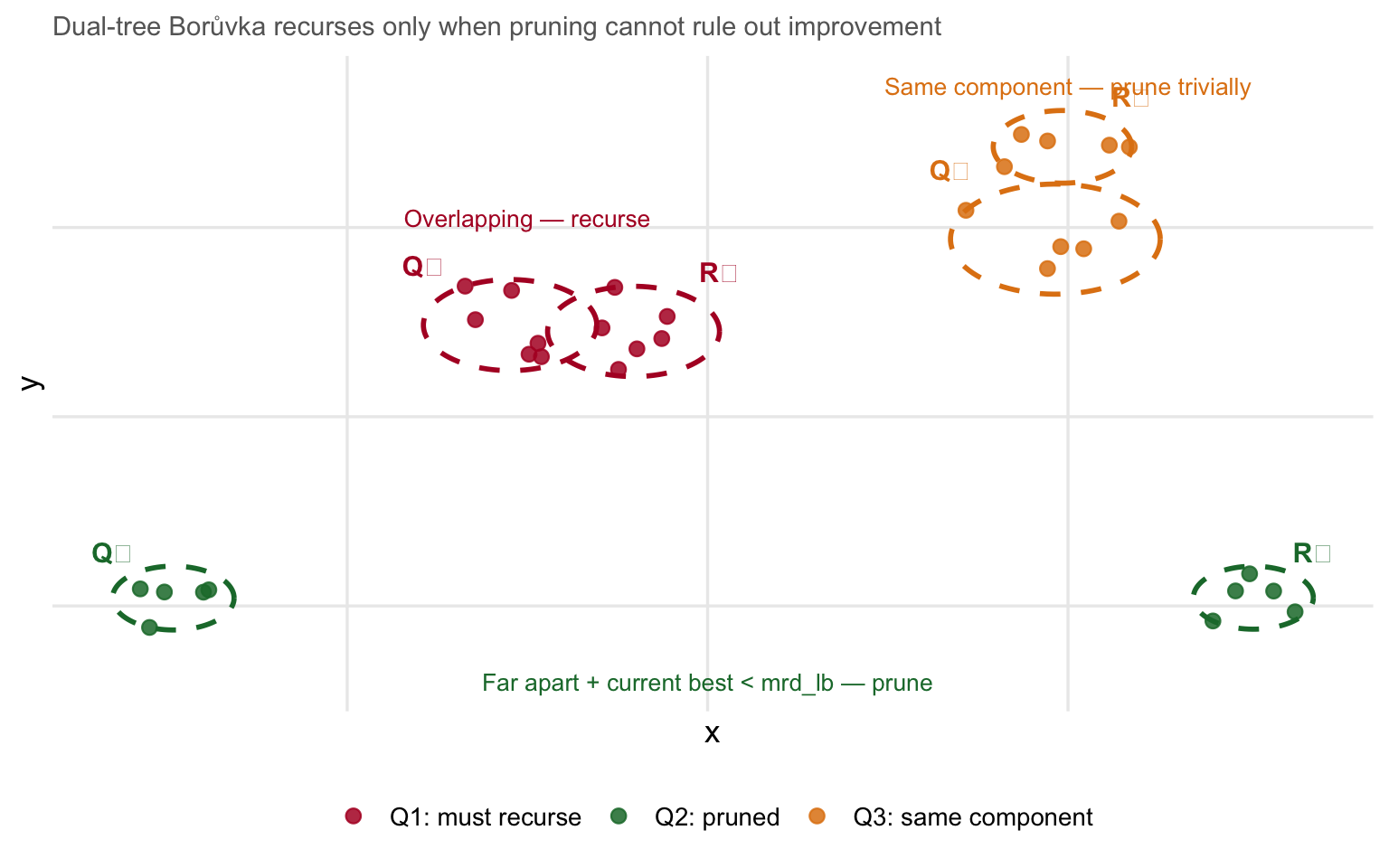
Dual-tree pruning. Red pair (Q₁, R₁): the balls overlap and mrd_lb is below the current best — must recurse. Green pair (Q₂, R₂): balls are well-separated; mrd_lb already exceeds every component’s current best edge — entire pair pruned. Orange pair (Q₃, R₃): same-component — trivially pruned.

7.2 The pruning condition

At every recursive call on subtree pair \((Q, R)\), the algorithm checks:

\[\text{mrd\_lb}(Q, R) \;\geq\; \max\bigl(\text{best}[Q],\; \text{best}[R]\bigr)\]

where \(\text{best}[\cdot]\) is the maximum current best outgoing edge weight across all components in that subtree.

If this holds, even the cheapest possible MRD edge between \(Q\) and \(R\) cannot improve any component in either subtree — the entire pair is skipped.

If it fails, the algorithm recurses into children, splitting the larger subtree, until leaf nodes are reached and actual point pairs are evaluated.

7.3 The warm-up

Before the first round, \(\text{best}[\text{every node}] = \infty\) — no pruning is possible and the first traversal degenerates to \(O(n^2)\) leaf-pair work.

Rhobots avoids this by reusing the kNN results from the core-distance pass as a warm-up. After the core-distance computation each point already knows its \(k = \text{min\_pts}+1\) nearest neighbours and their MRD values. These seed finite \(\text{best}\) values before Round 1, enabling tree pruning from the very first traversal.

---

8 From MST to Clusters: TRUE SPLIT vs Noise Fallout

Once the MST is complete, HDBSCAN processes its edges in ascending MRD order (root-to-leaves), tracking two events at each merge:

TRUE SPLIT — both sides of the merge have \(\geq \text{min\_pts}\) members. A new cluster pair is born; both children are tracked.

Noise fallout — one side is too small (\(< \text{min\_pts}\)). The small side’s points fall off as noise at this \(\lambda\) level; the cluster continues through the large side unchanged.

set.seed(12)
# MST with clear splits (two well-separated blobs)
g1_s <- cbind(rnorm(8, -2, 0.3), rnorm(8, 0, 0.3))
g2_s <- cbind(rnorm(7,  2, 0.3), rnorm(7, 0, 0.3))
X_s  <- rbind(g1_s, g2_s)
D_s  <- as.matrix(dist(X_s))
mst_s <- prim_mst(D_s)

# "Spine" MST: points arranged in a line, each merge adds 1 point
X_sp <- cbind(seq(-3, 3, length.out=15), rnorm(15, 0, 0.05))
D_sp <- as.matrix(dist(X_sp))
mst_sp <- prim_mst(D_sp)

draw_mst <- function(X, mst_obj, title_txt, subtitle_txt) {
  e <- mst_obj$edges; w <- mst_obj$w
  pts <- data.frame(x=X[,1], y=X[,2])
  segs <- data.frame(x0=X[e[,1],1], y0=X[e[,1],2],
                     x1=X[e[,2],1], y1=X[e[,2],2], w=w)
  ggplot() +
    geom_segment(data=segs, aes(x=x0,y=y0,xend=x1,yend=y1,colour=w),
                 linewidth=1.5) +
    geom_point(data=pts, aes(x,y), size=4, colour="grey20") +
    scale_colour_gradient(low="#4292C6", high="#FC4E2A", guide="none") +
    labs(title=title_txt, subtitle=subtitle_txt, x=NULL, y=NULL)
}

p_split <- draw_mst(X_s, mst_s,
  "TRUE SPLIT present",
  "Both sides of the central cut have ≥ 5 points → two real clusters")
p_spine <- draw_mst(X_sp, mst_sp,
  "Spine MST — no TRUE SPLIT",
  "Each merge adds 1 point < min_pts → all points fall off as noise; 1 root cluster")

grid.arrange(p_split, p_spine, ncol=2)

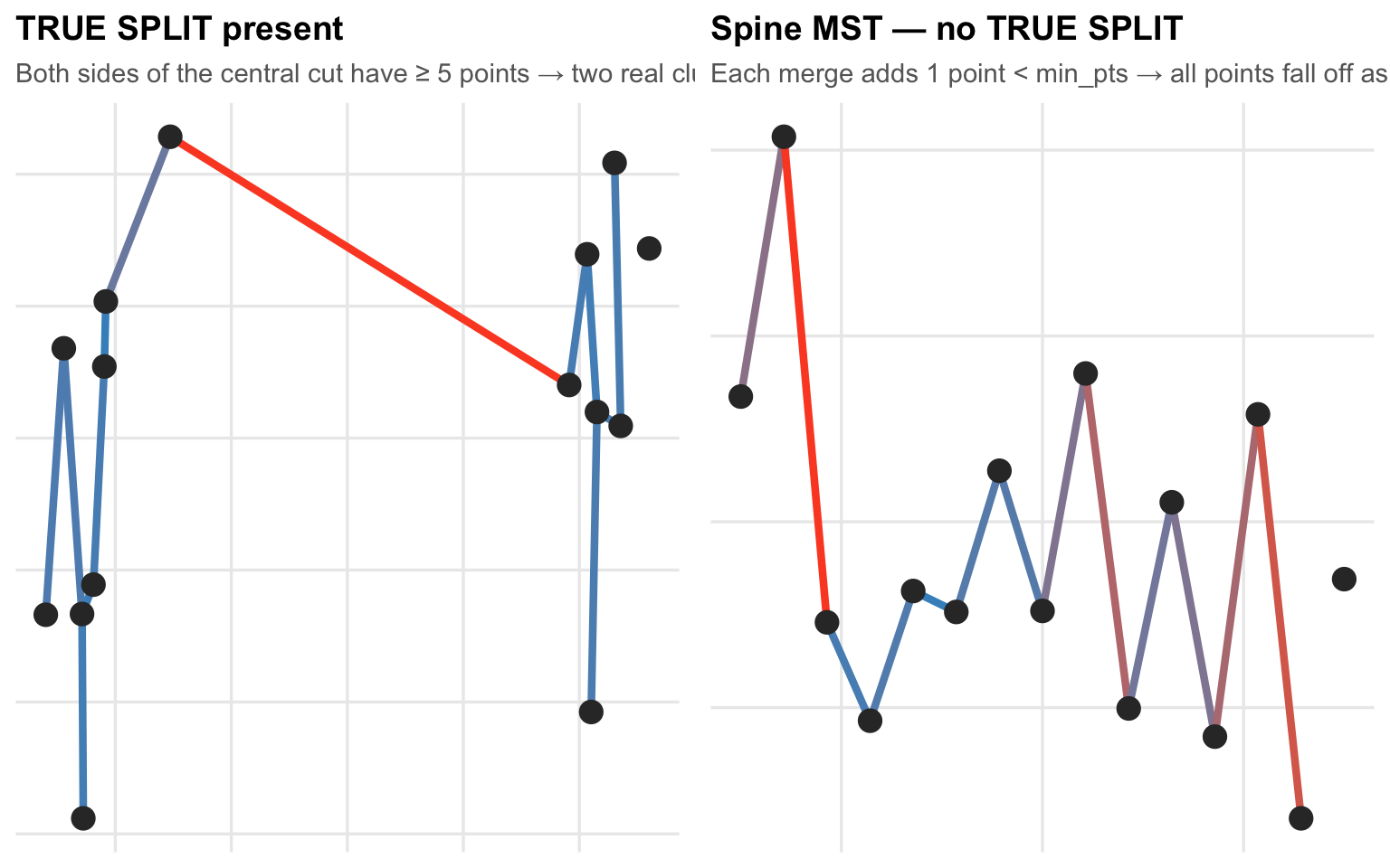
How the MST structure determines the condensed tree. Left: an MST with a clear TRUE SPLIT (both sides ≥ min_pts=5 at the cut). Right: a spine-shaped MST where every merge has one side < min_pts — no TRUE SPLIT ever occurs, so the condensed tree collapses to a single root cluster.

Why this matters. A spine-shaped MST produces a condensed tree with no TRUE SPLIT nodes. The root cluster is a leaf in the condensed tree (no children), so EOM always selects it as the single cluster — regardless of the allow_single_cluster setting.

The structural shape of the MST is therefore the primary determinant of the number of clusters HDBSCAN returns. This is why different MST algorithms on the same data can give radically different cluster counts.

---

9 Prim’s vs Borůvka: When They Diverge

On a complete graph with all distinct edge weights, every MST algorithm finds the same unique MST. The divergence appears in two scenarios:

Scenario 1 — Tied edge weights. If many pairs have exactly the same MRD (common on diffuse UMAP embeddings where \(d_{\text{mrd}}(i,j) \approx \max(\text{core}(i), \text{core}(j))\) for all nearby pairs), the MST is not unique. Prim’s and Borůvka choose from the tied edges in different orders and build structurally different spanning trees.

Scenario 2 — Approximate search. A kNN-limited Borůvka (the "adaptive" and "fixed" modes) may not find the globally cheapest edge from a component when that edge goes beyond the \(k\) nearest Euclidean neighbours. The dual-tree modes (BallTree, KDTree) avoid this by searching all pairs with pruning, not just kNN pairs.

set.seed(77)
n_diff <- 30
X_diff <- matrix(rnorm(n_diff * 2), n_diff, 2)   # pure noise: diffuse, no structure
D_diff <- as.matrix(dist(X_diff))
MIN_C  <- 4L
core_d <- apply(D_diff, 1, function(r) sort(r)[MIN_C + 1])
MRD    <- matrix(0, n_diff, n_diff)
for (i in seq_len(n_diff))
  for (j in seq_len(n_diff))
    MRD[i,j] <- max(core_d[i], core_d[j], D_diff[i,j])

# Prim's on full MRD
mst_prim <- prim_mst(MRD)

# Borůvka on full MRD (simulation)
boruvka_mst_full <- function(W) {
  n   <- nrow(W); par <- seq_len(n); sz <- rep(1L, n)
  find <- function(x) { while (par[x]!=x) { par[x]<<-par[par[x]]; x<-par[x] }; x }
  unite <- function(a,b) {
    ra<-find(a); rb<-find(b); if(ra==rb) return(FALSE)
    if(sz[ra]<sz[rb]) { tmp<-ra; ra<-rb; rb<-tmp }
    par[rb]<<-ra; sz[ra]<<-sz[ra]+sz[rb]; TRUE
  }
  edges <- matrix(0L,0,2); ws <- numeric(0)
  repeat {
    if (length(unique(sapply(seq_len(n),find)))==1) break
    bw<-rep(Inf,n); bu<-rep(-1L,n); bv<-rep(-1L,n)
    for(i in seq_len(n)) { ci<-find(i)
      for(j in seq_len(n)) { cj<-find(j); if(ci==cj) next
        if(W[i,j]<bw[ci]){bw[ci]<-W[i,j];bu[ci]<-i;bv[ci]<-j} } }
    for(r in seq_len(n)) { if(bu[r]<0) next
      if(unite(bu[r],bv[r])) { edges<-rbind(edges,c(bu[r],bv[r])); ws<-c(ws,bw[r]) } }
  }
  list(edges=edges, w=ws)
}
mst_bor <- boruvka_mst_full(MRD)

# Count TRUE SPLITS (both sides ≥ min_pts)
count_true_splits <- function(mst_obj, n, min_c) {
  e <- mst_obj$edges; w <- mst_obj$w
  ord <- order(w)
  e <- e[ord,,drop=FALSE]; w <- w[ord]
  comp <- seq_len(n); sz <- rep(1L,n)
  find <- function(x) { while(comp[x]!=x){comp[x]<<-comp[comp[x]];x<-comp[x]};x }
  splits <- 0L
  for (i in seq_along(w)) {
    ra<-find(e[i,1]); rb<-find(e[i,2])
    sa<-sz[ra]; sb<-sz[rb]
    if(sa>=min_c && sb>=min_c) splits <- splits+1L
    # merge
    if(sz[ra]>=sz[rb]){comp[rb]<-ra;sz[ra]<-sz[ra]+sz[rb]}
    else{comp[ra]<-rb;sz[rb]<-sz[rb]+sz[ra]}
  }
  splits
}

sp_prim <- count_true_splits(mst_prim, n_diff, MIN_C)
sp_bor  <- count_true_splits(mst_bor,  n_diff, MIN_C)

draw_mst2 <- function(X, mst_obj, title_txt) {
  e <- mst_obj$edges; w <- mst_obj$w
  pts <- data.frame(x=X[,1],y=X[,2])
  segs <- data.frame(x0=X[e[,1],1],y0=X[e[,1],2],
                     x1=X[e[,2],1],y1=X[e[,2],2],w=w)
  ggplot() +
    geom_segment(data=segs,aes(x=x0,y=y0,xend=x1,yend=y1,colour=w),linewidth=1.2) +
    geom_point(data=pts,aes(x,y),size=3,colour="grey30") +
    scale_colour_gradient(low="#4292C6",high="#FC4E2A",guide="none") +
    labs(title=title_txt, x=NULL, y=NULL)
}

p_p <- draw_mst2(X_diff, mst_prim,
  sprintf("Prim's: %d TRUE SPLITS (→ up to %d clusters)", sp_prim, sp_prim+1))
p_b <- draw_mst2(X_diff, mst_bor,
  sprintf("Borůvka: %d TRUE SPLITS (→ up to %d clusters)", sp_bor, sp_bor+1))
grid.arrange(p_p, p_b, ncol=2)

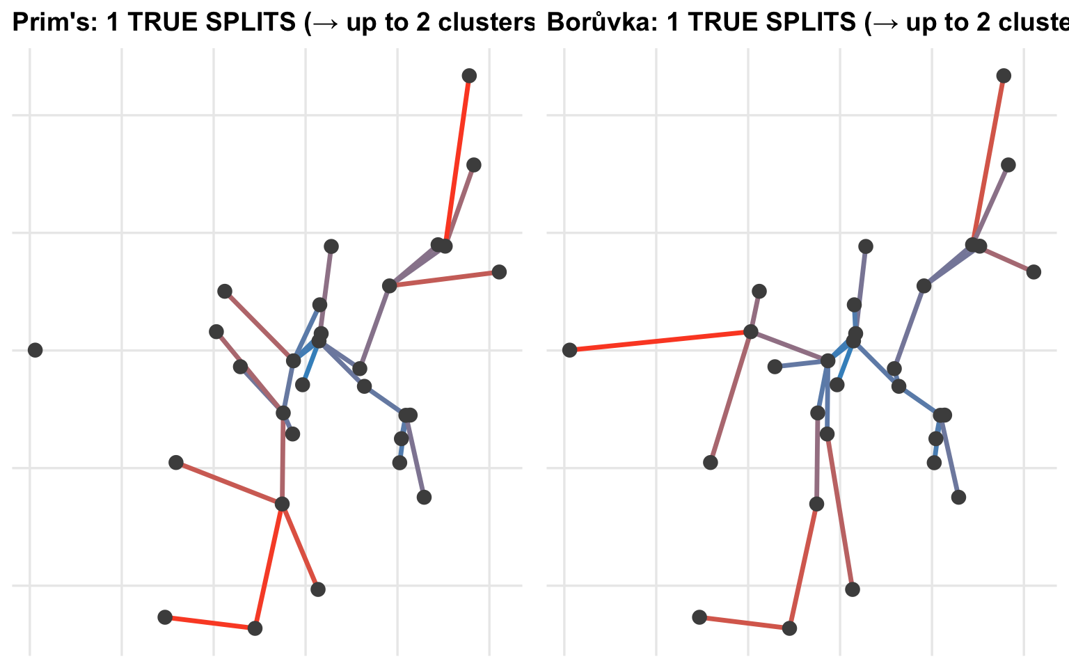
Prim’s vs Borůvka MSTs on a diffuse dataset where many MRD values are nearly equal. Both are valid spanning trees — same total weight — but their branching structure differs. Prim’s tree (left) has more balanced splits; Borůvka’s (right) tends toward a ‘greedy local’ structure. The resulting condensed trees can produce very different cluster counts.

Warning

Both MSTs are valid — but structurally different.

On diffuse data where many MRD values are close to each other, the tie-breaking order (determined by which algorithm sees pairs first) produces trees with very different numbers of TRUE SPLIT nodes.

This is the root cause of cluster-count differences between Rhobots’ Borůvka and Python’s Prim’s implementation on sentiment/emotion datasets: both find a minimum spanning tree, but one has more balanced branches (more TRUE SPLITS, more clusters) than the other.

The allow_single_cluster = FALSE parameter (default since Rhobots v0.1.7) mitigates this when the condensed tree has children but EOM would wrongly select only the root. It cannot help when the condensed tree genuinely has no TRUE SPLIT nodes.

---

10 allow_single_cluster = FALSE

Before v0.1.7, Rhobots could return a single cluster in two situations:

1. Genuinely unimodal data — the condensed tree has no children at the root. One cluster is the correct answer.

2. EOM selecting the root — the condensed tree has children, but the root cluster’s stability score exceeds the sum of its children’s stabilities. EOM picks the root, ignoring sub-structure that really is present.

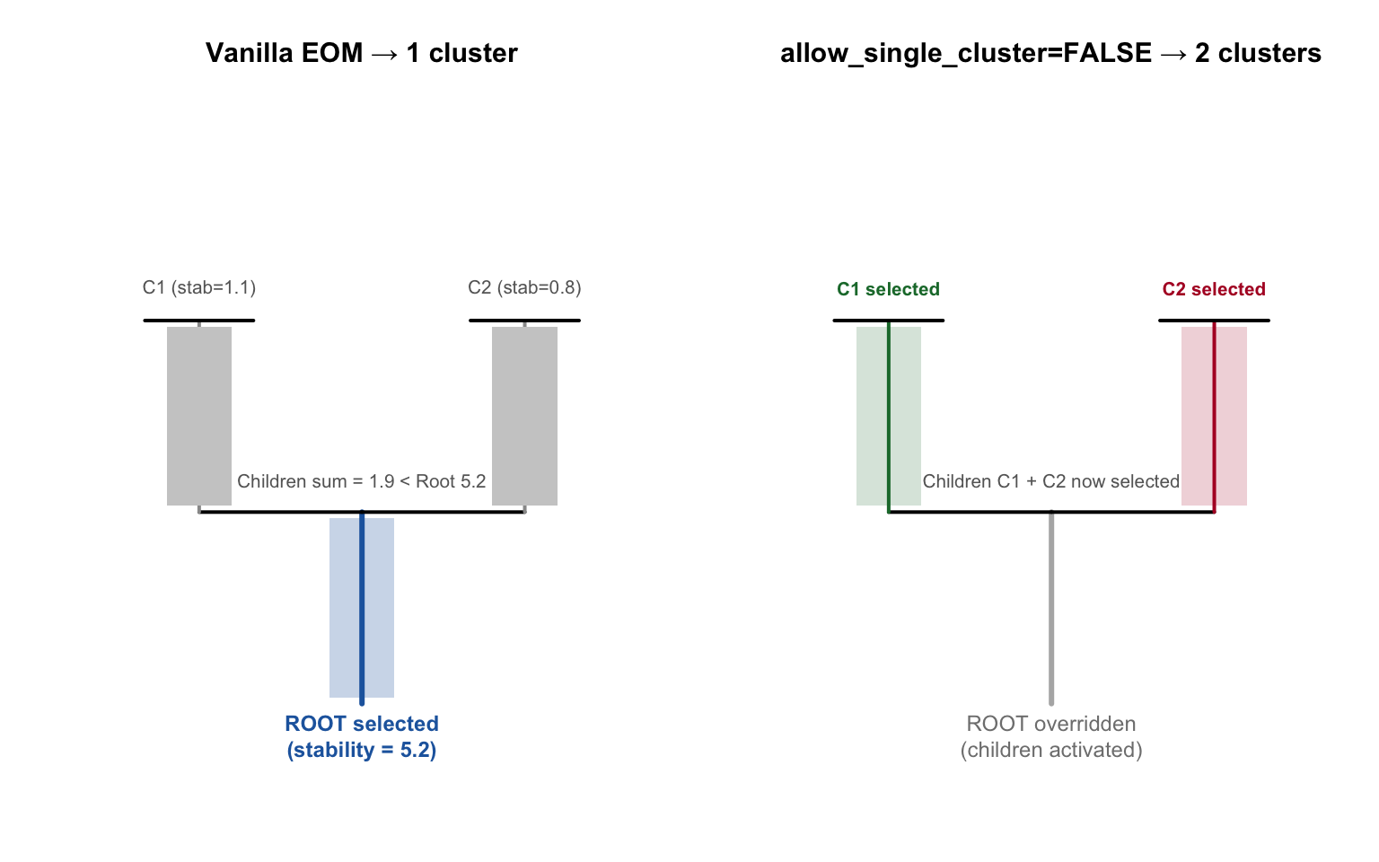
The allow_single_cluster = FALSE option (matching Python hdbscan’s default) handles case 2: if EOM would select only the root and the root has children, the selection restarts from the root’s children.

# Schematic illustration — base R
par(mfrow=c(1,2), mar=c(2,2,3,1))

# Left: EOM selects root
plot.new(); plot.window(xlim=c(0,10), ylim=c(0,10))
title("Vanilla EOM → 1 cluster", cex.main=0.95)
segments(5,1,5,4,lwd=3,col="#2166AC")          # root
segments(5,4,2,4,lwd=2); segments(5,4,8,4,lwd=2)
segments(2,4,2,7,lwd=2,col="grey60"); segments(8,4,8,7,lwd=2,col="grey60")
segments(2,7,1,7,lwd=2); segments(2,7,3,7,lwd=2)
segments(8,7,7,7,lwd=2); segments(8,7,9,7,lwd=2)
rect(4.4,1.1,5.6,3.9, col="#2166AC40", border=NA)
rect(1.4,4.1,2.6,6.9, col="grey80", border=NA)
rect(7.4,4.1,8.6,6.9, col="grey80", border=NA)
text(5,0.5,"ROOT selected\n(stability = 5.2)",col="#2166AC",cex=0.75,font=2)
text(2,7.5,"C1 (stab=1.1)",col="grey40",cex=0.65)
text(8,7.5,"C2 (stab=0.8)",col="grey40",cex=0.65)
text(5,4.5,"Children sum = 1.9 < Root 5.2",col="grey40",cex=0.65)

# Right: allow_single_cluster=FALSE overrides root
plot.new(); plot.window(xlim=c(0,10), ylim=c(0,10))
title("allow_single_cluster=FALSE → 2 clusters", cex.main=0.95)
segments(5,1,5,4,lwd=3,col="grey70")
segments(5,4,2,4,lwd=2); segments(5,4,8,4,lwd=2)
segments(2,4,2,7,lwd=2,col="#1B7837")
segments(8,4,8,7,lwd=2,col="#B2182B")
segments(2,7,1,7,lwd=2); segments(2,7,3,7,lwd=2)
segments(8,7,7,7,lwd=2); segments(8,7,9,7,lwd=2)
rect(1.4,4.1,2.6,6.9, col="#1B783730", border=NA)
rect(7.4,4.1,8.6,6.9, col="#B2182B30", border=NA)
text(5,0.5,"ROOT overridden\n(children activated)",col="grey50",cex=0.75)
text(2,7.5,"C1 selected",col="#1B7837",cex=0.65,font=2)
text(8,7.5,"C2 selected",col="#B2182B",cex=0.65,font=2)
text(5,4.5,"Children C1 + C2 now selected",col="grey40",cex=0.65)

How allow_single_cluster=FALSE works. In the condensed tree (left), root stability (blue bar) exceeds the sum of children’s stabilities, so vanilla EOM returns 1 cluster. With allow_single_cluster=FALSE (right), the root is overridden and children are activated — returning 3 clusters.

par(mfrow=c(1,1))

---

11 Computational Complexity

Phase	Operation	Complexity	Notes
Core distances	kNN search × \(n\)	\(O(n \log n)\)	Shared with Borůvka warm-up
Warm-up	MRD for \(k\) neighbours per point	\(O(nk)\)	Seeds finite best values
Borůvka round	Dual-tree traversal	\(O(n \log n)\)¹	Pruning depends on dimension
Rounds total	\(\lceil \log_2 n \rceil\) rounds	\(O(n \log^2 n)\)	Empirically close to linear
SL tree build	Sort \(n-1\) edges, Union-Find	\(O(n \log n)\)	Negligible
Condensed tree	One pass over SL tree	\(O(n)\)	Negligible
EOM extraction	Bottom-up + top-down	\(O(n)\)	Negligible

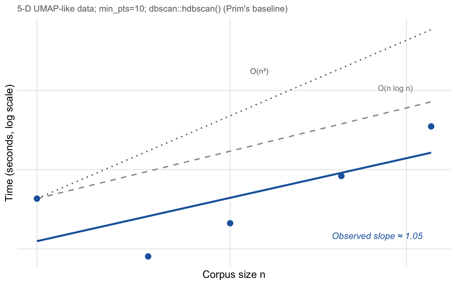
¹ The \(O(n \log n)\) per-round claim holds in low dimensions (2–3-D) where ball-tree pruning is nearly perfect. In 5-D UMAP space, pruning is partial: the algorithm is faster than \(O(n^2)\) but not yet \(O(n \log n)\). Empirical scaling on 5-D data is roughly \(O(n^{1.4})\) to \(O(n^{1.7})\).

set.seed(42)
ns_c  <- c(300, 600, 1000, 2000, 3500)
times <- sapply(ns_c, function(n) {
  X <- matrix(rnorm(n * 5), n, 5)
  system.time(dbscan::hdbscan(X, minPts = 10L))[["elapsed"]]
})

timing_c <- data.frame(n = ns_c, t = times)
fit_lm   <- lm(log(t) ~ log(n), data = timing_c)
slope    <- round(coef(fit_lm)[2], 2)

ref_n  <- c(min(ns_c), max(ns_c))
ref_ln <- data.frame(
  n      = ref_n,
  t_nlogn = times[1] * (ref_n / ns_c[1]) * log(ref_n) / log(ns_c[1]),
  t_n2    = times[1] * (ref_n / ns_c[1])^2
)

ggplot(timing_c, aes(n, t)) +
  geom_line(data=ref_ln, aes(n, t_nlogn), colour="grey60",
            linetype="dashed", linewidth=0.8) +
  geom_line(data=ref_ln, aes(n, t_n2), colour="grey40",
            linetype="dotted", linewidth=0.8) +
  geom_point(size=3, colour="#2166AC") +
  geom_smooth(method="lm", se=FALSE, colour="#2166AC", linewidth=1.2) +
  annotate("text", x=2800, y=ref_ln$t_nlogn[2]*1.5,
           label="O(n log n)", colour="grey50", size=3.5) +
  annotate("text", x=1200, y=ref_ln$t_n2[2]*0.3,
           label="O(n²)", colour="grey40", size=3.5) +
  annotate("text", x=2500, y=times[3]*0.7,
           label=paste0("Observed slope ≈ ", slope),
           colour="#2166AC", size=4, fontface="italic") +
  scale_x_log10(labels=scales::comma) +
  scale_y_log10(labels=function(x) paste0(x,"s")) +
  labs(x="Corpus size n", y="Time (seconds, log scale)",
       subtitle="5-D UMAP-like data; min_pts=10; dbscan::hdbscan() (Prim's baseline)")

Empirical HDBSCAN runtime scaling on 5-D synthetic data. Log-log scale; slope ≈ 1.5 indicates sub-quadratic but super-linear growth in 5-D. The dashed reference lines show ideal O(n log n) and quadratic O(n²) scaling.

---

12 Summary

Concept	What it does
MST	\(n-1\) edges connecting all points with minimum total MRD weight
Borůvka round	Every component simultaneously finds its cheapest outgoing edge
Union-Find	Tracks component membership in O(α(n)) per query
MRD lower bound	Allows pruning subtree pairs that cannot improve any component
Dual-tree pruning	Ball-tree geometry eliminates O(log n) subtree pairs per point
Warm-up	Reuses kNN from core-distance pass to enable pruning in Round 1
TRUE SPLIT	Merge where both sides ≥ min_pts → new cluster born in condensed tree
Noise fallout	Merge where one side < min_pts → small side exits as noise
allow_single_cluster=FALSE	If EOM picks only root but root has children, override to children

Three things to remember about the MST and cluster counts:

1. The MST structure, not just its weight, determines cluster counts. A balanced binary MST has many TRUE SPLIT nodes → many clusters. A spine-shaped MST has none → always 1 cluster from EOM.

2. On diffuse data, many MRD values are nearly equal. The MST is not unique. Prim’s (greedy global) and Borůvka (parallel local) break ties differently, producing structurally different trees and different cluster counts.

3. allow_single_cluster=FALSE fixes EOM over-aggregation but not MST shape. It helps when the condensed tree has children that EOM ignores. It cannot create TRUE SPLITS that the MST never produced.